DATA473
Algorithms in Data Science
Alex Gavryushkin
Table of contents
- Lecture 1: Background
- Lecture 2: Turing machines
- Lecture 3: Universal Turing machine
- Lecture 4: Recursive functions, halting problem
- Lecture 5: Kolmogorov complexity
- Lecture 6: Properties of Kolmogorov complexity
- Lecture 7: Basic algorithms recap
- Lecture 8: Sorting
- Lecture 9: NP-hard problems
- Lecture 10: Proving NP-hardness
- Lecture 11: AI for discovering new algorithms
- Lecture 12: AlphaDev
Literature, resources
- These slides
- Complementary (rapidly evolving) lecture notes
- Tim Roughgarden: Algorithms Illuminated
- Papers including these that we will use:
Biological Data Science Lab @UCNZ
GitHub: @bioDS
Twitter: @bioDS_lab
Introduction

ML = Machine Learning
CoSt = Computational Statistics
AS = Applied Statistics

Garey and Johnson. Computers and Intractability. 1979
Why biological data science?
Because the skills are highly transferable:
- Scale
- Heterogeneity
- Visualisation and communication
- High-performance computing
Why is it suddenly a thing?

Lecture 1: Background
Finite state automata
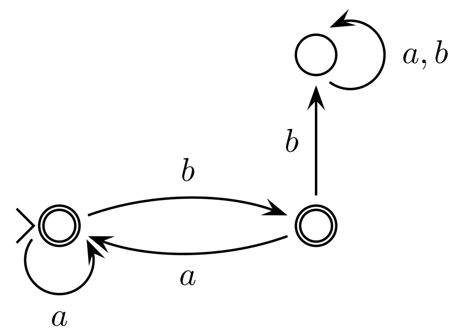
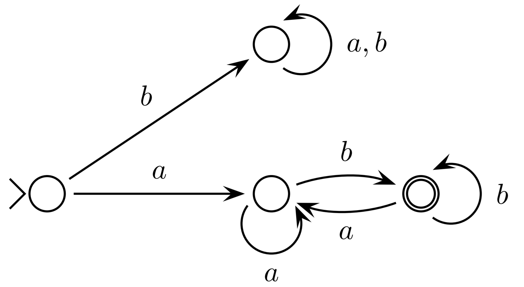

DFA = NFA
Pumping Lemma
Lecture 2: Turing machines
- A finite set $\Gamma$ called the alphabet (or tape symbols)
- A finite set $Q$ of states
- A distinguished state $q_0 \in Q$ called the starting state
- A subset $F \subseteq Q$ of halting states
- A distinguished symbol $\beta \in \Gamma$ called the blank symbol (or the empty cell)
- A partial function $F: (Q \setminus F) \times \Gamma \to Q \times \Gamma \times \{L, R, \varnothing\}$
called the programme
The program does not terminate otherwise.
Hence a non-terminating programme either hangs (infinite loop) or crashes (reaches a state and tape symbol with no command to execute).
We will be starting Turing machines on $$ \beta\underset{\Delta}{a_1} a_2 \ldots a_n \beta $$
$$ \begin{align} \mbox{Example 2} &\\ & q_0 \beta \to \mathrm{accept} \beta\\ & q_0 0 \to q_0 \beta R\\ & q_0 1 \to q_0 \beta R \end{align} $$
$$ \begin{align} \mbox{Example 3} &\\ & q_0 \beta \to \mathrm{accept} \beta\\ & q_0 0 \to q_0 1 R\\ & q_0 1 \to q_0 0 R \end{align} $$
for all $x$ and $y$: $$ f(x) = y $$ $$ \Updownarrow $$ $$ \beta \underbrace{1 \ldots 1}_{x \mbox{ times}} \beta \Rightarrow_M \beta \underbrace{1 \ldots 1}_{y \mbox{ times}} \beta \mbox{ and $M$ halts} $$
We denote the latter by $M(x) = y$.
We write $M(x)\downarrow$ for $M$ halts on $\beta \underbrace{1 \ldots 1}_{x \mbox{ times}} \beta$
for all $x_1, x_2$, and $y$: $$ f(x_1, x_2) = y $$ $$ \Updownarrow $$ $$ \beta \underbrace{1 \ldots 1}_{x_1 \mbox{ times}} 0 \underbrace{1 \ldots 1}_{x_2 \mbox{ times}} \beta \Rightarrow_M \beta \underbrace{1 \ldots 1}_{y \mbox{ times}} \beta \mbox{ and $M$ halts} $$ Similarly for more than two variables $x_1, x_2, \ldots, x_n$.
Example 2: implement the following module COPY. $$ \beta \underbrace{1 \ldots 1}_{x \mbox{ times}} \beta \Rightarrow_M \beta \underbrace{1 \ldots 1}_{x \mbox{ times}} 0 \underbrace{1 \ldots 1}_{x \mbox{ times}} \beta $$
Example 3: compute: $$ f(x, y) = xy $$
$a^* b^*$
$\{a^n b^n \mid n \in \mathbb N\}$
Church–Turing thesis
A problem can be solved by an algorithm if and only if it can be solved by a Turing machine.Universal Turing Machine
Theorem: There exists a Turing Machine $U$ which computes all computable functions.That is, for every computable function $f(x)$ there exists a number $s$ such that $U(s, x) = y$ if and only if $f(x) = y$.

Turing machine
Lecture 3: Universal Turing machine
Theorem: There exists a universal Turing Machine $U$.
That is, for every Turing Machine $M(\bar x)$ there exists a number $s$ such that $U(s, \bar x) = y$ if and only if $M(\bar x) = y$.
Proof
Idea 1: $s$ is $M$'s "number"
Idea 2: $U$ "decodes" $s$ into $M$'s program
Idea 3: $U$ "simulates" $M$'s execution on $\bar x$
Trick 1: Recursive functions
Trick 2: Multi-tape Turing machines
Lecture 4: Recursive functions, halting problem
Primitive recursive functions
Partial recursive functions
Recursive function that is not primitive recursive
Halting problem
Theorem: Not everything is computable.For example, the following function is not computable $$ h(x) = \begin{cases} U(x, x) + 1, & \mbox{ if } U(x, x) \downarrow\\ 0, & \mbox{ otherwise} \end{cases} $$

Lecture 5: Kolmogorov complexity

https://learn.canterbury.ac.nz/course/view.php?id=19467
Definition
Kolmogorov complexity $K(\bar x)$ of string $\bar x$ is $$\min {\{|M_s| ~\bigg |~ U(s, 0) = \bar x\}}$$ where $U$ is a universal Turing machine.Theorem
The definition is invariant under the programming language, that is, $K_U(\bar x) \leq K_A (\bar x) + c_A$ for every algorithm $A$.
Given two languages $A$ and $B$ and a compression algorithm $M$, we say that $M$ is good if $$|M(A, B)| \leq |M(A)| + |M(B)| + c$$
With the idea of (unsupervised) model pre-training in mind, what is the best compression algorithm?
Kolmogorov complexity as the ultimate goal for compressors
And neural network training is effectively a search for such compressor.Lecture 6: Properties of Kolmogorov complexity
Definition
Kolmogorov complexity $K(x)$ of a string $x$ is $$\min {\{|M_s| ~\bigg |~ U(s, 0) = x\}}$$ where $U$ is a universal Turing machine.Theorem
The following problems cannot be solved by an algorithm:- Algorithm triviality
- Algorithm equivalence
- Kolmogorov complexity
Theorem
Properties of $K(x)$:- For all $x, K(x) \leq |x| + c$
- $K(xx) = K(x) + c$
- $K(1^n) \leq O(\log n)$
- $K(1^{n!}) \leq O(\log n)$
- $K(xy) \leq K(x) + K(y) + O(\log(\min\{K(x), K(y)\}))$ (compare with the definition of "good compression algorithm")
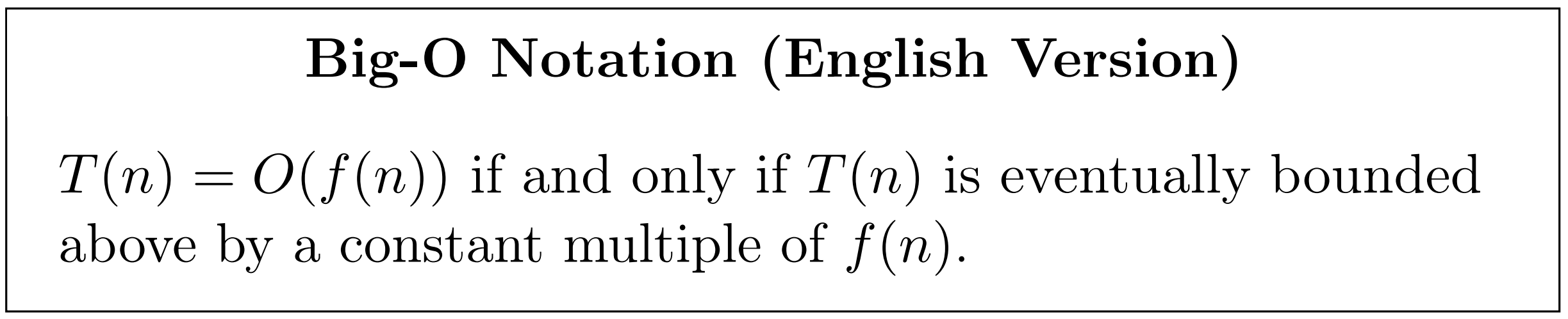
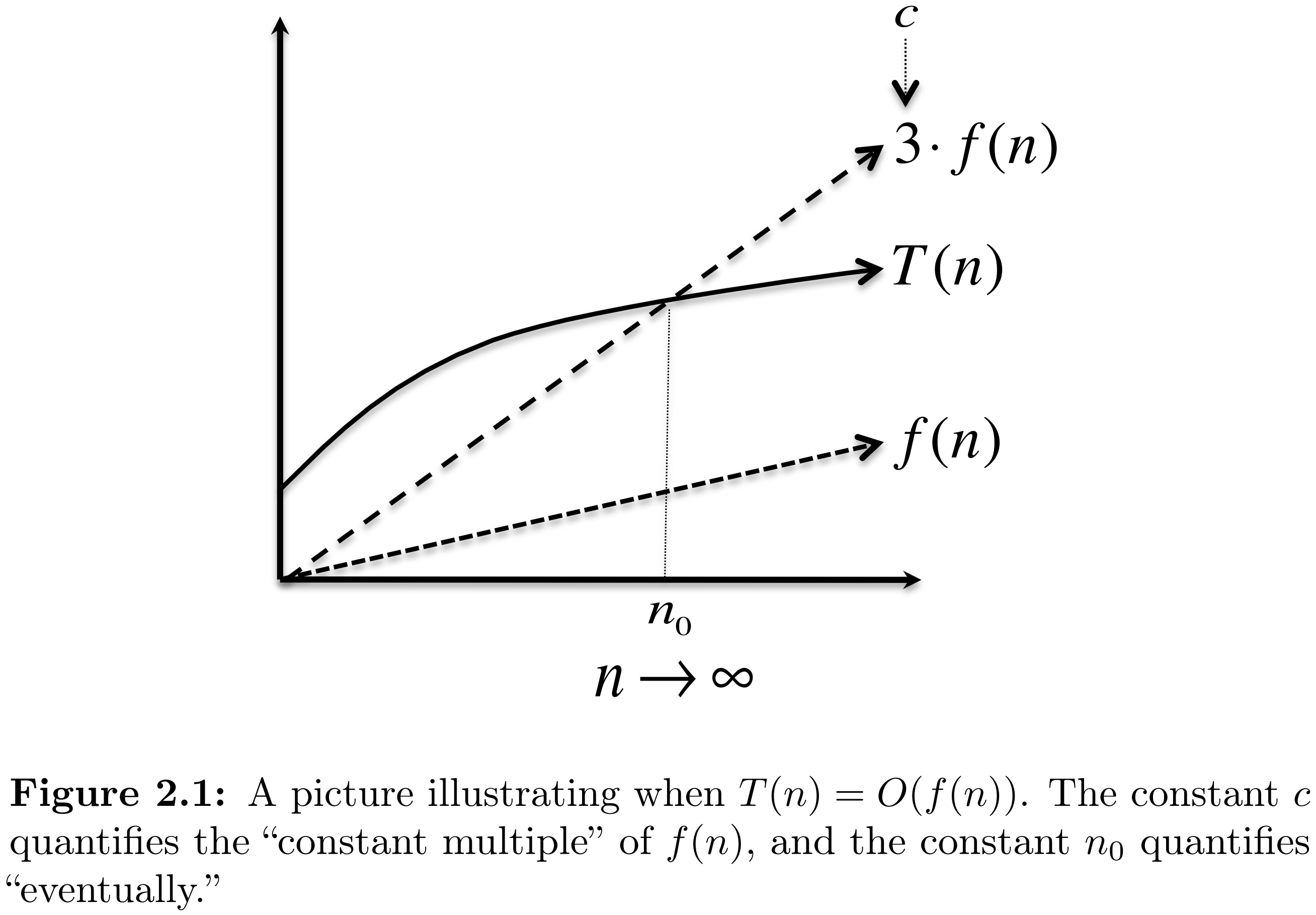
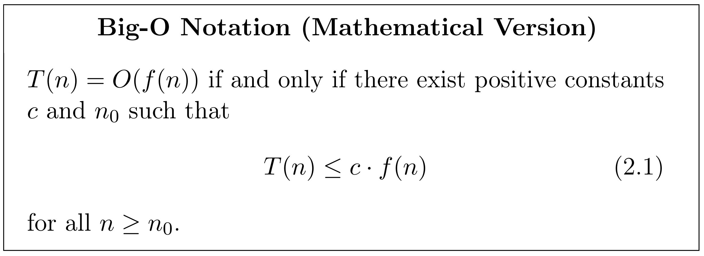
Big O notation recap
Chapters 2.1 and 2.2 in Roughgarden's Algorithms Illuminated Part 1.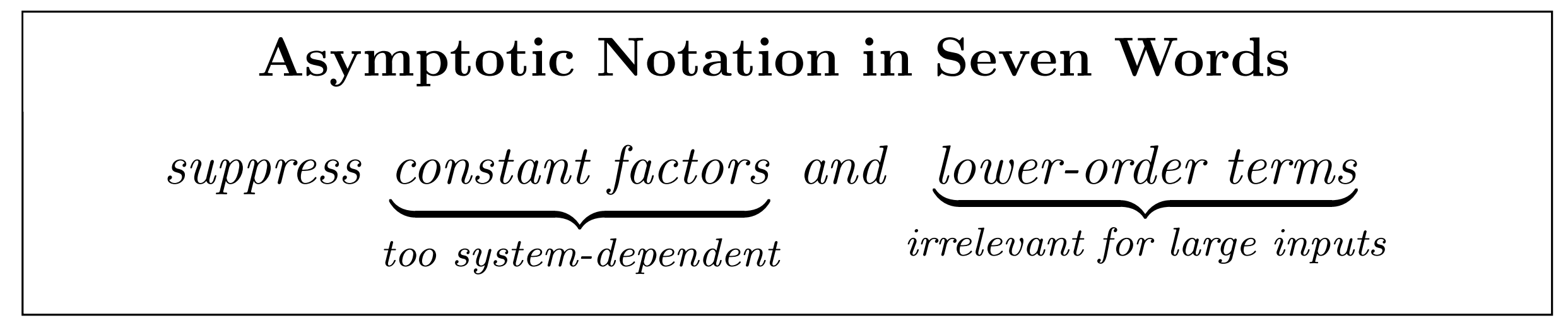
Conditional Kolmogorov complexity: connection to pre-training
$K(x|y)$ is the length of the smallest TM that generates $x$ given $y$.Properties:
- $K(x|\varnothing) = K(x)$
- $K(x|x) = c$
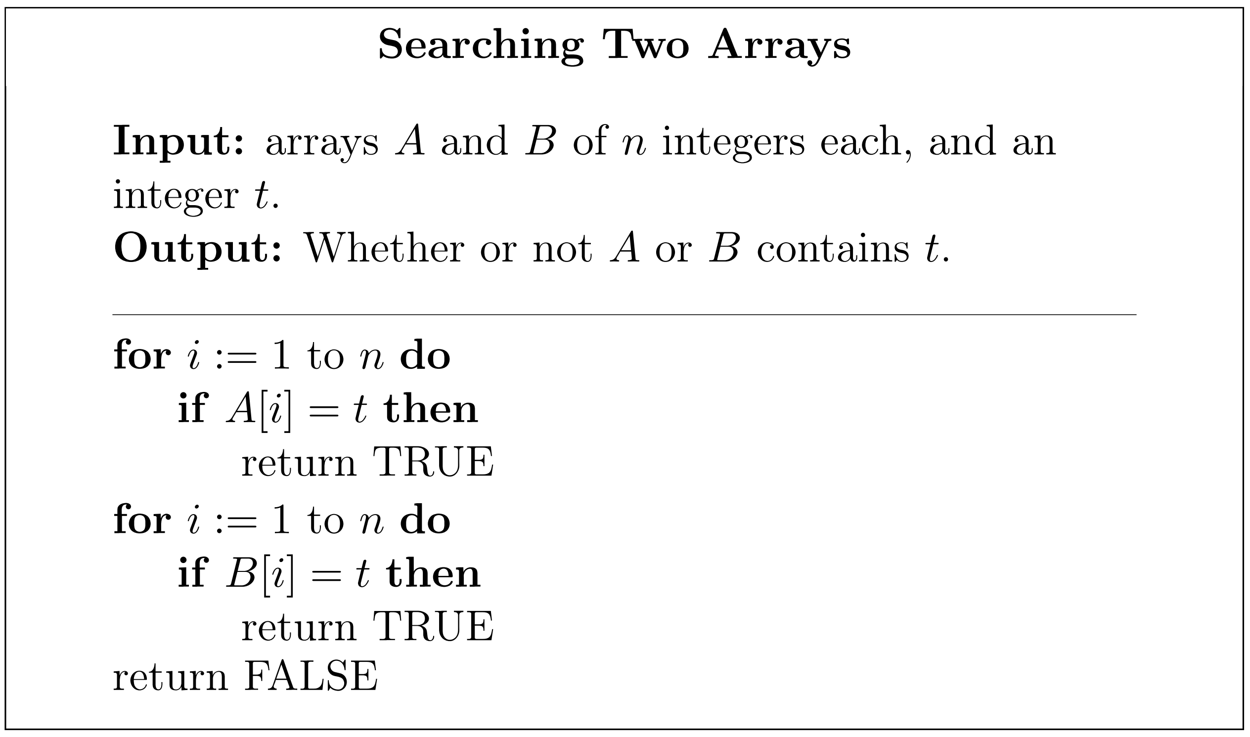
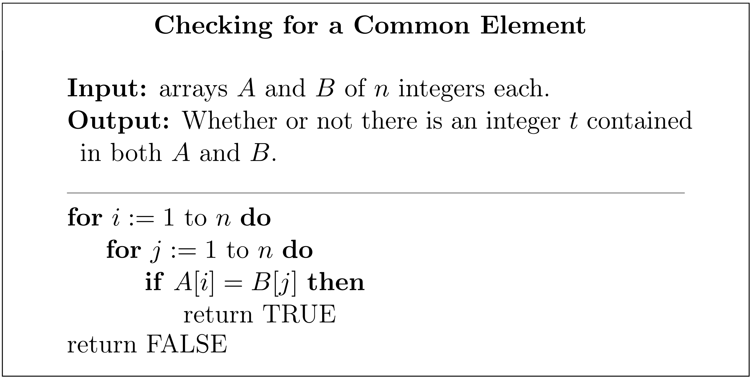
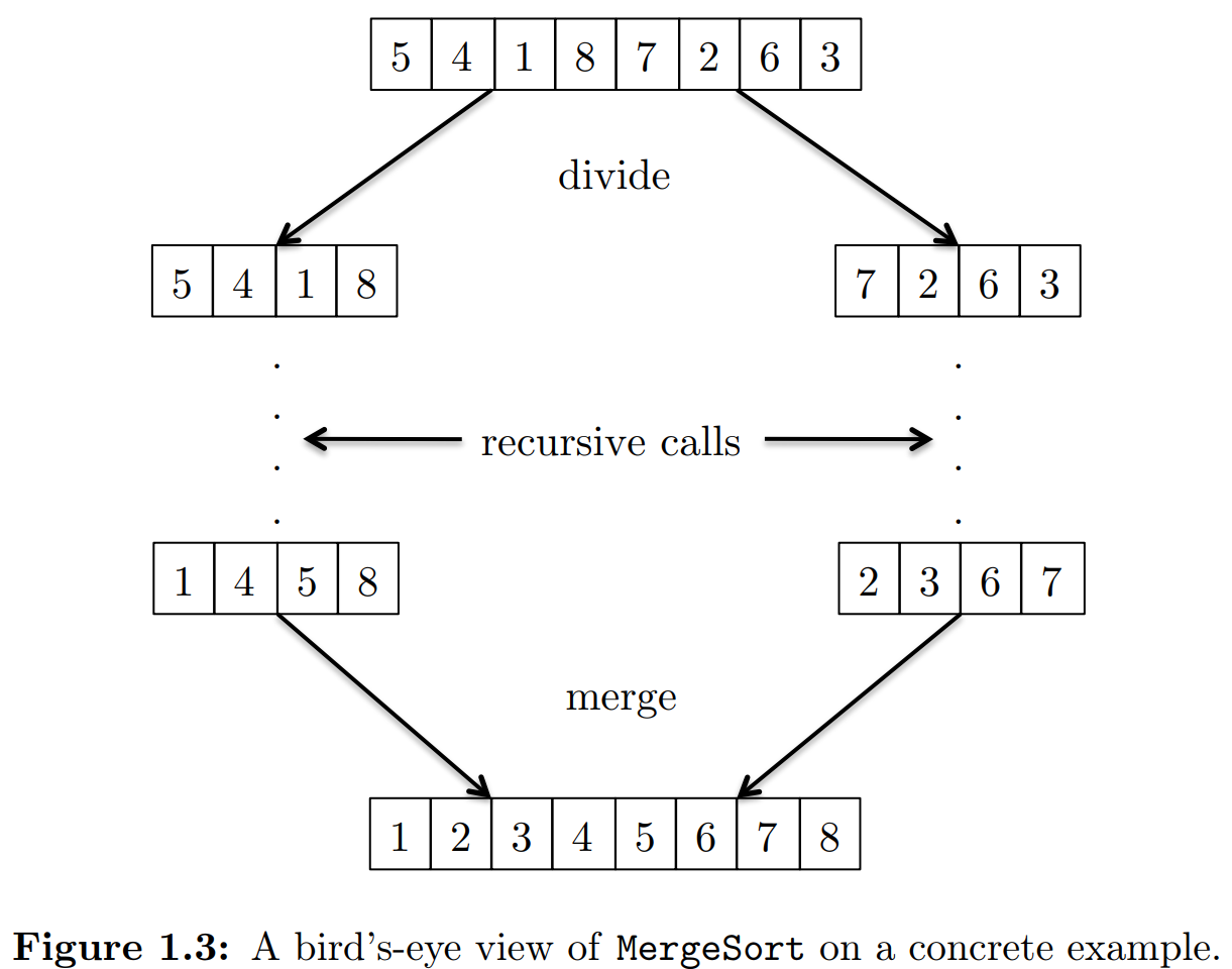
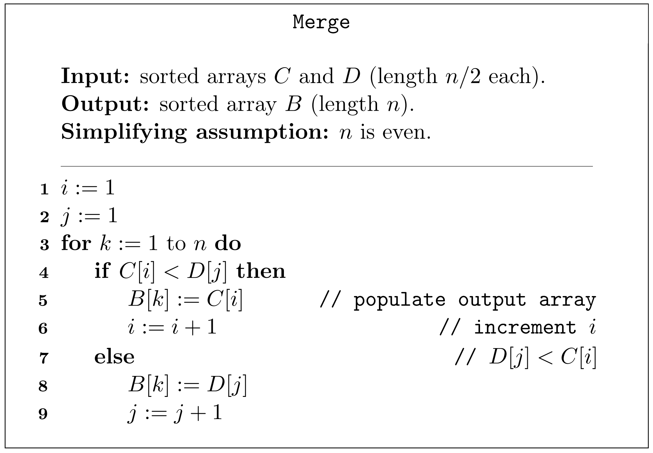
$\mathtt{MergeSort}$
Running time of $\mathtt{MergeSort}$
Theorem 1.2 For every input array of length $n \geq 1$, the $\mathtt{MergeSort}$ algorithm performs at most $$ 6n\log_2 n + 6n $$ operations, where $log_2$ denotes the base-2 logarithm.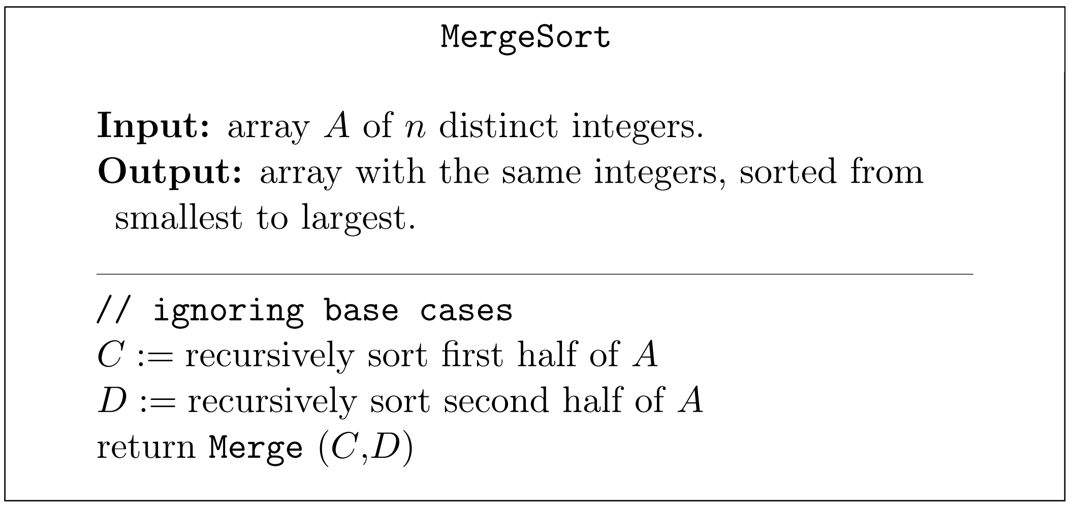
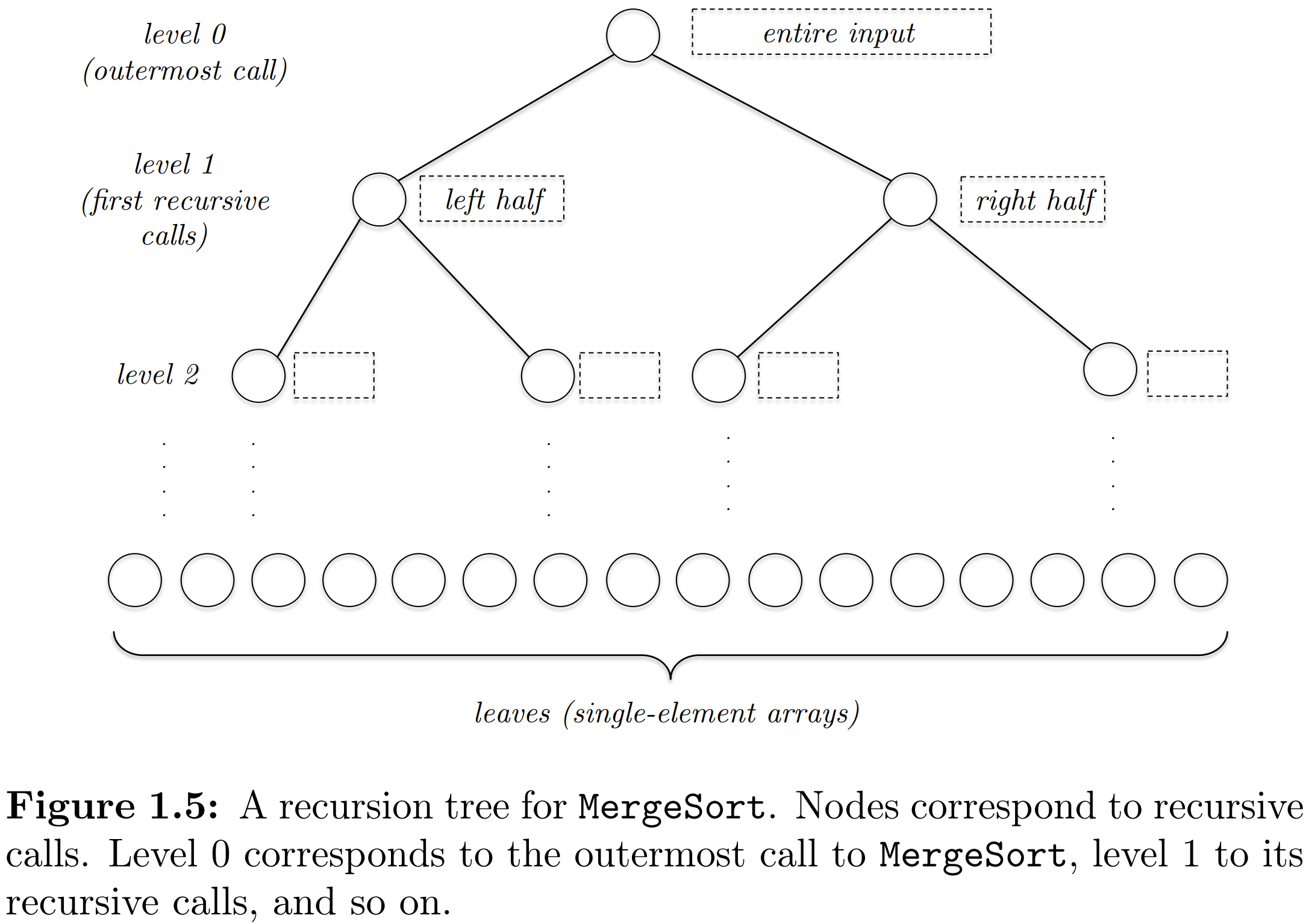
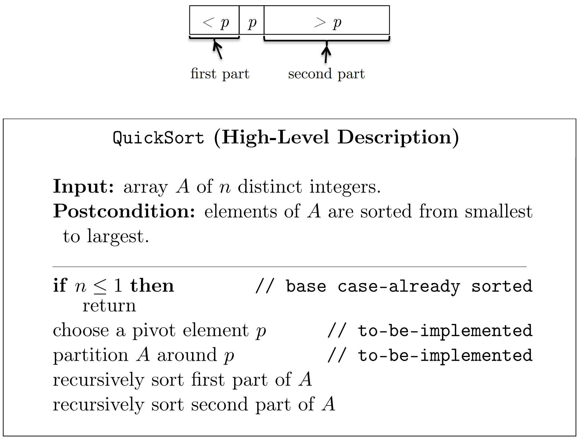
The divide-and-conquer paradigm
- Divide the input int smaller subproblems
- Conquer the subproblems recursively
- Combine the solution for the subproblems into a solution for the original problem
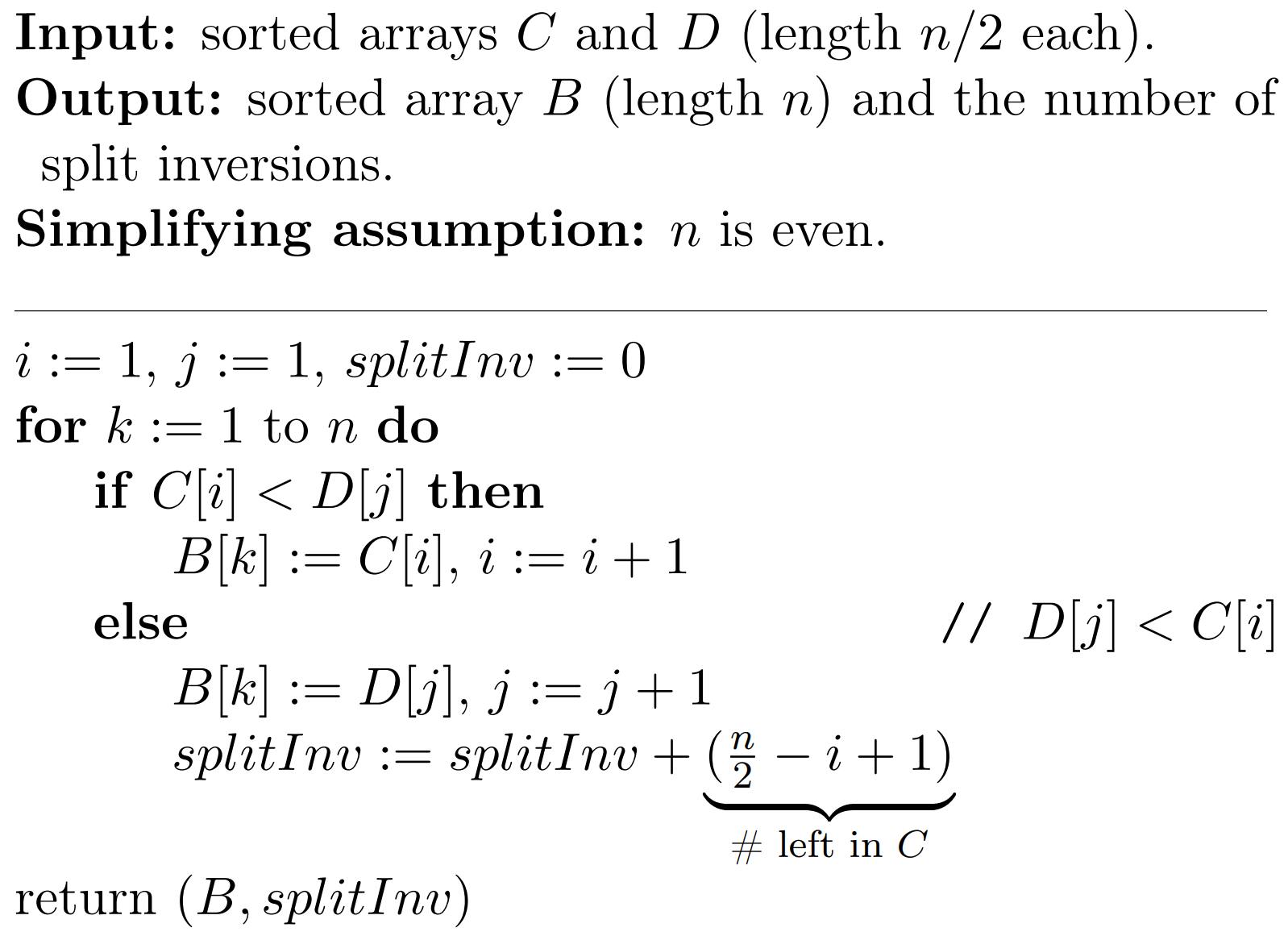
Compare with $\mathtt{Merge}$

Example
\begin{align} & x_1 \vee x_2 \vee x_3 & \neg x_1 \vee \neg x_2 \vee x_3 \\ & \neg x_1 \vee x_2 \vee x_3 & \neg x_1 \vee x_2 \vee \neg x_3 \\ & x_1 \vee \neg x_2 \vee x_3 & x_1 \vee \neg x_2 \vee \neg x_3 \\ & x_1 \vee x_2 \vee \neg x_3 & \neg x_1 \vee \neg x_2 \vee \neg x_3 \\ \end{align}Three facts about NP-hard problems
- Ubiquity: Practically relevant NP-hard problems are everywhere.
- Intractability: Under a widely believed mathematical conjecture, no NP-hard problem can be solved by any algorithm that is always correct and always runs in polynomial time.
- Not a death sentence: NP-hard problems can often (but not always) be solved in practice, at least approximately, through sufficient investment of resources and algorithmic sophistication.
Three properties (you can't have them all)
- General-purpose. The algorithm accommodates all possible inputs of the computational problem.
- Correct. For every input, the algorithm correctly solves the problem.
- Fast. For every input, the algorithm runs in polynomial time.
Rookie mistakes
- Thinking that "NP" stands for "not polynomial".
- Saying that a problem is "an NP problem" or "in NP" instead of "NP-hard".
- Thinking that NP-hardness doesn't matter because NP-hard problems can generally be solved in practice.
- Thinking that advances in computer technology will rescue us from NP-hardness.
- Devising a reduction in the wrong direction.
Acceptable inaccuracies
- Assuming that the P$\ne$NP conjecture is true.
- Using the terms "NP-hard" and "NP-complete" interchangeably.
- Conflating NP-hardness with requiring exponential time in the worst case.