COSC341

Theory of Computing

Alex Gavryushkin

Lecture 1

Introduction

Who cares about theory of computing?
I do!

ML = Machine Learning
CoSt = Computational Statistics
AS = Applied Statistics

Who cares about theory of computing?
You do!

Garey and Johnson. Computers and Intractability.

Why biological data science?

Because the skills are highly transferable:

• Noisy data
• Visualisation
• Communication
• High-performance computing

Why is it suddenly a thing?

Sets

Empty set
$\varnothing$
is a set!

Operations on sets

ML = Data $\cap$ Algorithms

(Statistics$\setminus$DS) $\cap$ Algorithms $\neq \varnothing$

$\overline{\mbox{Data} \cup \mbox{Algorithms} \cup \mbox{Statistics}} = ?$

Lecture 2

Sets, relations, functions

Subsets, ordered tuples, relations, and functions

$A \subseteq B \iff (\forall x) (x \in A \Rightarrow x \in B)$

$\mathcal P(A) = \{X \mid X \subseteq A\}$

$(a, b) = (c, d) \iff (a = c~\&~b = d)$

$A \times B = \{(a, b) \mid a \in A, b \in B\}$

$P \subseteq A \times B$ is a relation (from $A$ to $B$, or on $A$ if $A = B$)

$f \subseteq A \times B$ is a function if $(f(a) = b ~\&~ f(a) = c) \Rightarrow b = c$

Types of functions

injective if $f(a) = f(b) \Rightarrow a = b$

surjective if $(\forall y \in B)(\exists x \in A)f(x) = y$

bijective if $f$ is injective and surjective.

Molecular biology: crash course

Classical genetics

Modern genomics

Reality

Partitions and equivalence relations

$A = B \sqcup C$ is a partition if $A = B \cup C$ and $B \cap C = \varnothing$

A relation $\sim$ on $A$ is called an equivalence relations if $\sim$ is:

• Reflexive $(\forall x \in A)~x \sim x$
• Symmetric $(\forall x, y \in A)~(x \sim y \Rightarrow y \sim x)$
• Transitive $(\forall x, y, z \in A)~(x \sim y ~\&~ y \sim z \Rightarrow x \sim z)$

Theorem 1

1. A partition $A_1 \sqcup A_2 \sqcup \ldots$ of the set $A$ is defined by an equivalence relation on $A$.
2. An equivalence relation $\sim$ on the set $A$ defines a partition on $A$.

Lecture 3

Cardinality

Set $A$ has smaller cardinality than $B$ if there exists a (total) injection $f : A \to B$, written $|A| \leqslant |B|$.

Theorem: $|A| = |B| \iff (|A| \leqslant |B| ~\&~ |B| \leqslant |A|)$.

$|\mathbb N| \stackrel{?}{=} |\mathbb Z| \stackrel{?}{=} |\mathbb Q| \stackrel{?}{=} |\mathbb R|$

Theorem 2

Lecture 4

Finite state automata

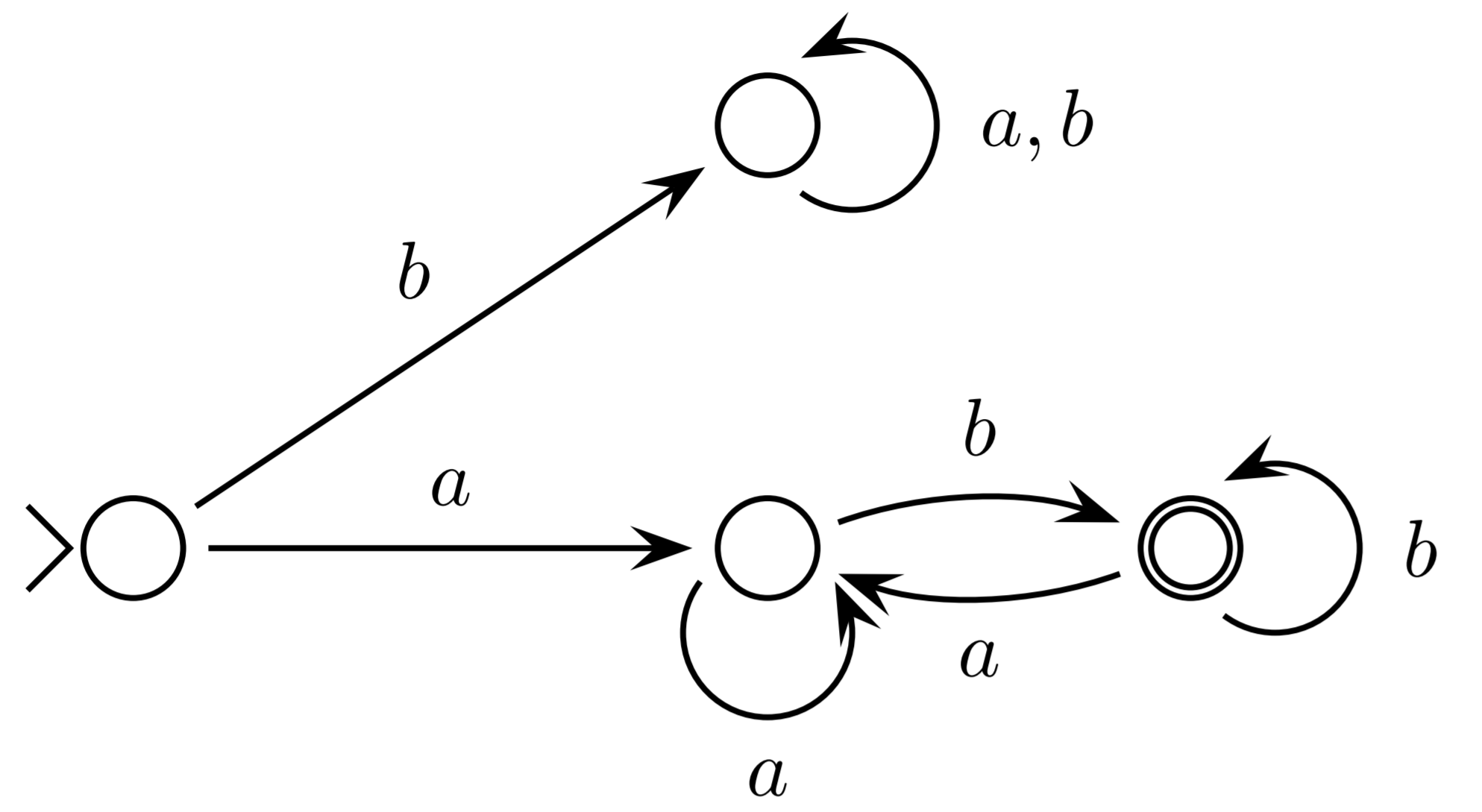
DFA

• A finite set, $Q$, of states
• A finite set $\Sigma$ called the alphabet
• A total function $\delta: Q \times \Sigma \to Q$ called the transition function
• A distinguished state $q_0 \in Q$ called the initial state
• A subset $F \subseteq Q$ called the final or accepting states.

We say that $M$ accepts or recognises $w$ if $q_n \in F$ and otherwise it rejects $w$.

The language of $M$, $L(M)$ is just the set of strings in $\Sigma^*$ that $M$ accepts.

Lecture 5

Non-deterministic automata

NFA

$\{ab\}$ in English alphabet

Examples

Design an automaton that recognises the following languages in alphabet $\{a,b\}$

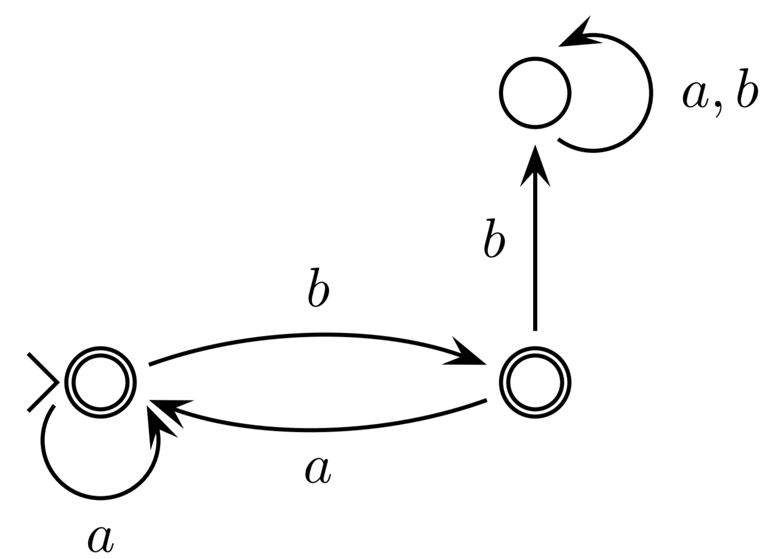
$L_1 = \{w | w = xaaybbbz, \mbox{ where } x,y,z \in\{a,b\}^*\}$

$L_2 = \{w | w \mbox{ contains $aa$ or $bbb$}\}$

$L_3 = \{w | w \mbox{ contains $aa$ and $bbb$}\}$

Lecture 6

NFA = DFA, pumping lemma

Theorem 3

Theorem 3

Lecture 7

Pumping lemma

Pumping lemma

Let $L$ be an automatic language. Then there exists a positive integer $k$ such that if $z \in L$, $|z| \geq k$ then for some $u$, $v$, and $w$:
$ \begin{eqnarray*} z &=& u \cdot v \cdot w \\ |u| + |v| &\leq& k \\ |v| &>& 0 \\ uv^iw &\in& L \quad \mbox{for all $i \geq 0$}. \end{eqnarray*} $

Proof: Haven't we just proven it?

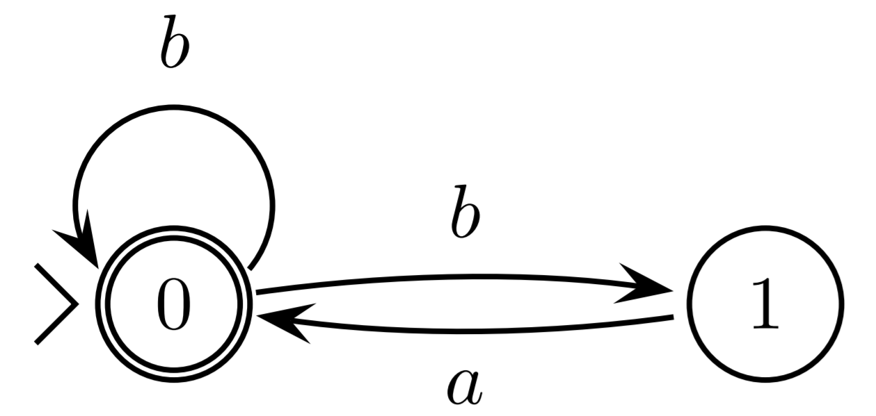
$L = \{w \in \{a, b\} \mid \mbox{$w$ contains an odd number of $a$'s}$
$\mbox{and an even number of $b$'s}\}$

Lecture 8

Pushdown automata and context free grammars

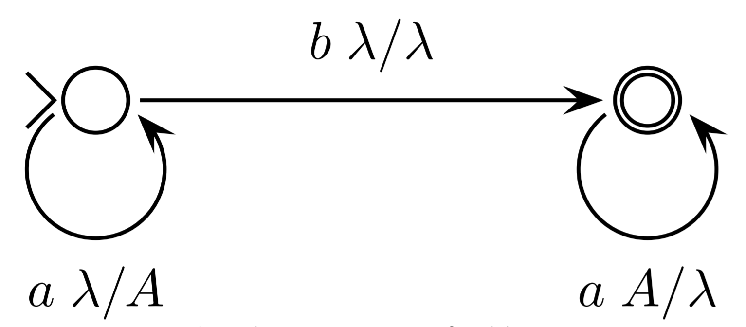
• A finite set $Q$ of states
• A finite set $\Sigma$ called the input alphabet (lower case letters)
• A finite set $\color{blue}{\Gamma}$ called the stack alphabet (upper case letters)
• A relation $\delta \subseteq Q \times \Sigma \cup \{\lambda\} \times \color{blue}{\Gamma \cup \{\lambda\}} \times Q \times \color{blue}{\Gamma \cup \{\lambda\}}$
  called the transition relation
• A distinguished state $q_0 \in Q$ called the initial state
• A subset $F \subseteq Q$ called the final or accepting states.

The stack should be empty to accept a string!

• A finite set $V$ of nonterminals (or variables)
  (upper case letters)
• A finite set $\Sigma$ called the alphabet (or terminals)
  (lower case letters), $\Sigma \cap V = \varnothing$
• A finite set $P$ of production rules,
  which is a subset of $V \times (V \cup \Sigma)^*$
• A distinguished $S \in V$ called the start symbol

Examples
$S \to aS, S \to bS, S \to \lambda$

$S \to aS, S \to bT, T \to bT, T \to \lambda$

$\{a^nb^n \mid n \in \mathbb{N}\}$

Theorem

Genome phasing

Schwarz, Roland F., Anne Trinh, Botond Sipos, James D. Brenton, Nick Goldman, and Florian Markowetz. 2014. “Phylogenetic Quantification of Intra-Tumour Heterogeneity.” PLoS Computational Biology 10 (4): e1003535.

Schwarz, Roland F., Anne Trinh, Botond Sipos, James D. Brenton, Nick Goldman, and Florian Markowetz. 2014. “Phylogenetic Quantification of Intra-Tumour Heterogeneity.” PLoS Computational Biology 10 (4): e1003535.

Lecture 9

Regular languages

If $\alpha$ and $\beta$ are regular expressions then so are the following:
$(\alpha\beta)$; $(\alpha \cup \beta)$; $\alpha^*$

The language $L_\alpha$ described by the regular expression $\alpha$ is defined in the following way:
$L_\alpha = \varnothing$ if $\alpha = \varnothing$
$L_\alpha = \{\lambda\}$ if $\alpha = \lambda$
$L_\alpha = \{x\}$ if $\alpha = x$

$L_{\alpha\beta} = \{uv \mid u \in L_\alpha \mbox{ and } v \in L_\beta\}$
$L_{\alpha\cup\beta} = L_\alpha \cup L_\beta$
$L_{\alpha^*} = \{w_1 \ldots w_k \mid w_1, \ldots, w_k \in L_\alpha \mbox{ and } k \in \mathbb N\}$

Language $L$ is called regular if it can be described by a regular expression $\alpha$, that is, there exists $\alpha$ such that $L = L_\alpha$.

Examples

Lecture 10

Classification of languages, Pumping Lemma 2

Proof: Easy.

Theorem (ii): Automatic languages are closed under
$\cdot$ (concatenation), $\cup$ (union), $\cap$ (intersection),
and $\overline{\phantom a}$ complement.

Proof: Even easier.

Theorem (iii): Context-free languages are closed under
$\cdot$ (concatenation) and $\cup$ (union),
but not $\cap$ (intersection) or $\overline{\phantom a}$ complement.

Proof: Not yet possible — we need a version of the pumping lemma.

Classification of languages

Pumping Lemma 2

Proof: Super easy now.

Note: However, if $L$ is a context-free language and $R$ a regular language then $L \cap R$ is context-free!

Lectures 11–13

Turing Machines

Turing machine

• A finite set $\Gamma$ called the alphabet (or tape symbols)
• A finite set $Q$ of states
• A distinguished state $q_0 \in Q$ called the starting state
• A subset $F \subseteq Q$ of halting states
• A distinguished symbol $\beta \in \Gamma$ called the blank symbol (or the empty cell)
• A partial function $F: (Q \setminus F) \times \Gamma \to Q \times \Gamma \times \{L, R, \varnothing\}$
  called the programme

Turing machines can be used to formalise all kinds of algorithmic problems, including language recognition, generation, etc.

Hence a non-terminating programme either hangs (infinite loop) or crashes (reaches a state and tape symbol with no command to execute).

We will be starting Turing machines on $$ \beta\underset{\Delta}{a_1} a_2 \ldots a_n \beta $$

$$ \begin{align} \mbox{Example 2} &\\ & q_0 \beta \to \mathrm{accept} \beta\\ & q_0 0 \to q_0 \beta R\\ & q_0 1 \to q_0 \beta R \end{align} $$

$$ \begin{align} \mbox{Example 3} &\\ & q_0 \beta \to \mathrm{accept} \beta\\ & q_0 0 \to q_0 1 R\\ & q_0 1 \to q_0 0 R \end{align} $$

We denote the latter by $M(x) = y$.
We write $M(x)\downarrow$ for $M$ halts on $\beta \underbrace{1 \ldots 1}_{x \mbox{ times}} \beta$

Example 2: implement the following module COPY. $$ \beta \underbrace{1 \ldots 1}_{x \mbox{ times}} \beta \Rightarrow_M \beta \underbrace{1 \ldots 1}_{x \mbox{ times}} 0 \underbrace{1 \ldots 1}_{x \mbox{ times}} \beta $$

Example 3: compute: $$ f(x, y) = xy $$

$a^* b^*$

$\{a^n b^n \mid n \in \mathbb N\}$

Universal Turing Machine

Halting problem